Introduction: The High Cost of Data Labeling

In the world of machine learning, data is often called the new oil, but there's a critical catch: this oil needs refining. For supervised learning models to work effectively, they require labeled data – examples that have been carefully annotated by human experts. This labeling process is notoriously expensive and time-consuming. According to industry surveys, companies spend an average of $50,000 to $100,000 labeling data for a single machine learning project, with some complex computer vision projects exceeding $500,000 in labeling costs alone.

Traditional approaches to data labeling follow a simple but inefficient pattern: collect as much data as possible, then label everything. This "label-first, ask-questions-later" approach has several problems. First, it wastes resources on labeling redundant or irrelevant examples. Second, it often leads to imbalanced datasets where easy-to-label examples are overrepresented. Third, and most importantly, it assumes all data points are equally valuable for training, which is rarely true in practice.

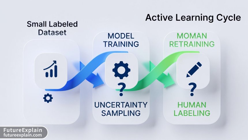
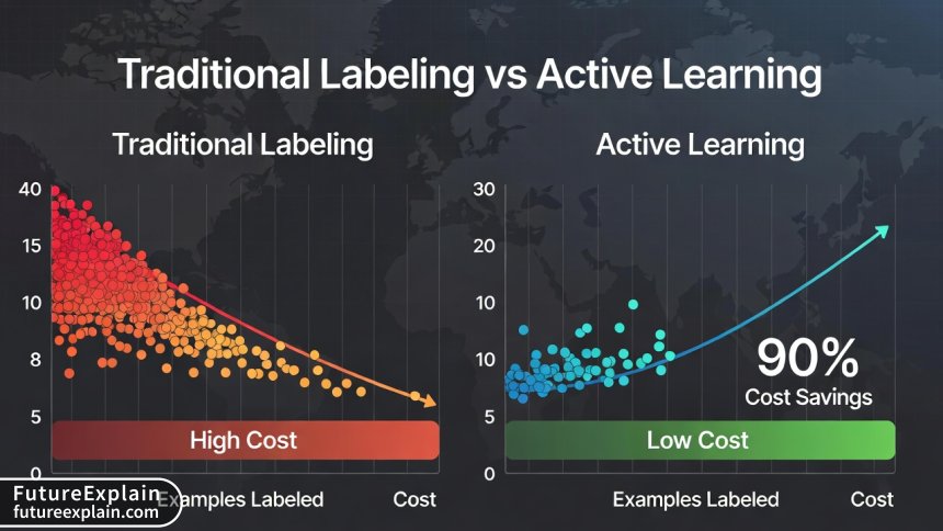
Active learning offers a smarter alternative. Instead of labeling everything upfront, active learning starts with a small labeled dataset, trains an initial model, and then strategically selects the most informative unlabeled examples for human annotation. This iterative process continues until the model reaches the desired performance level or the labeling budget is exhausted. The results can be dramatic: companies typically reduce labeling costs by 50-70% while often achieving better model performance than with traditional approaches.

What Is Active Learning? A Simple Analogy

Imagine you're trying to learn a new language. You have two options for study materials: Option A gives you 100 random sentences to translate. Option B gives you 10 carefully selected sentences, then asks you which concepts you find most confusing, and gives you more practice specifically on those difficult areas. Which approach would help you learn faster and more efficiently? Most people would choose Option B because it focuses effort where it's needed most.

Active learning applies this same principle to machine learning. The algorithm acts like a smart student who knows what they don't know. After learning from initial examples, the model identifies which additional examples would be most helpful to learn from next. These "informative" examples are then presented to human labelers, creating a feedback loop where each new labeled example provides maximum learning value.

The core insight behind active learning is that not all data is created equal. Some examples are redundant – if you've seen one picture of a cat from a certain angle, you've essentially seen dozens of similar cat pictures. Other examples are ambiguous or represent edge cases that the model finds confusing. By focusing labeling efforts on these ambiguous, uncertain, or representative examples, active learning achieves better performance with fewer labeled examples.

How Active Learning Actually Works: The Technical Foundation

At its core, active learning is an iterative process that alternates between model training and strategic data selection. The process typically follows these steps:

1. Initialization: Start with a small set of labeled data (the "seed set") and a larger pool of unlabeled data
2. Model Training: Train a machine learning model on the currently labeled data
3. Query Strategy: Use the trained model to evaluate the unlabeled pool and select the most informative examples
4. Human Labeling: Send the selected examples to human labelers for annotation
5. Iteration: Add the newly labeled examples to the training set and retrain the model
6. Stopping Criteria: Continue until reaching a performance threshold or exhausting the labeling budget

The magic happens in step 3 – the query strategy. This is where different active learning approaches diverge based on how they define "informative." The most common query strategies include:

Uncertainty Sampling

Uncertainty sampling selects examples where the current model is most uncertain about the correct label. For classification tasks, this often means choosing examples where the predicted probabilities are closest to uniform distribution across classes. For example, in a binary classification problem, uncertainty sampling would prioritize examples where the model predicts Class A with 51% probability and Class B with 49% probability, rather than examples with 99% confidence in either class.

Mathematically, uncertainty is often measured using:

• Least Confidence: 1 - P(ŷ|x) where ŷ is the most likely class
• Margin Sampling: The difference between the probabilities of the top two classes
• Entropy: -Σ P(y|x) log P(y|x) across all classes

Uncertainty sampling is particularly effective when the decision boundary between classes is complex and the model needs more examples near that boundary to understand it properly.

Query-by-Committee

Query-by-committee (QBC) maintains multiple models (a "committee") with different initializations or architectures. The algorithm selects examples where the committee members disagree most about the correct label. This approach leverages the "wisdom of crowds" principle – if multiple models trained on the same data disagree about an example, that example likely contains information that would help resolve their disagreement.

There are several ways to implement QBC:

• Version Space: Train multiple models that are consistent with the current labeled data
• Bagging: Train models on different bootstrap samples of the labeled data
• Architectural Diversity: Use different model architectures (CNN, Transformer, etc.)

The disagreement between committee members can be measured using:

• Vote Entropy: How evenly distributed the votes are across classes
• Kullback-Leibler Divergence: How much the predictions differ from the average
• Consensus Method: Select examples where no clear majority exists

Expected Model Change

Expected model change selects examples that would cause the greatest change to the current model if they were labeled and added to the training set. The intuition is that examples that would significantly alter the model's parameters must contain important information that the model currently lacks.

This approach is computationally expensive because it requires estimating how the model would change for each candidate example. However, approximations using gradient information or influence functions can make it practical. Expected model change tends to select diverse examples that cover different aspects of the problem space.

Density-Weighted Methods

Pure uncertainty sampling can sometimes select outliers or noisy examples that aren't representative of the broader data distribution. Density-weighted methods address this by combining uncertainty with representativeness. They select examples that are both uncertain and located in dense regions of the feature space.

The most common approach is to multiply an uncertainty score by a density estimate:

Score(x) = Uncertainty(x) × Density(x)^β

Where β controls the trade-off between uncertainty and representativeness. Density is typically estimated using kernel density estimation or nearest neighbor methods.

Practical Implementation: A Step-by-Step Guide

Now that we understand the theory, let's look at how to implement active learning in practice. We'll walk through a complete example using Python and popular machine learning libraries.

Step 1: Setting Up Your Environment

First, install the necessary libraries. For this example, we'll use scikit-learn, modAL (an active learning library), and matplotlib for visualization:

pip install scikit-learn modAL matplotlib numpy pandas

ModAL (Modular Active Learning) is a particularly useful library because it provides a flexible, modular framework for implementing active learning strategies with scikit-learn compatible estimators.

Step 2: Preparing Your Data

Active learning requires three datasets: a small initial labeled set, a large pool of unlabeled data, and a separate test set for evaluation. Here's how to set this up:

import numpy as np
from sklearn.datasets import make_classification
from sklearn.model_selection import train_test_split

# Generate synthetic data for demonstration
X, y = make_classification(
    n_samples=10000,
    n_features=20,
    n_informative=15,
    n_redundant=5,
    n_classes=3,
    random_state=42
)

# Split into initial labeled (1%), unlabeled pool (79%), and test set (20%)
X_labeled, X_pool, y_labeled, y_pool = train_test_split(
    X, y, train_size=0.01, random_state=42, stratify=y
)

X_pool, X_test, y_pool, y_test = train_test_split(
    X_pool, y_pool, train_size=0.95, random_state=42, stratify=y_pool
)

print(f"Initial labeled set: {len(X_labeled)} examples")
print(f"Unlabeled pool: {len(X_pool)} examples")
print(f"Test set: {len(X_test)} examples")

For real-world datasets, you'll need to adapt this approach. For image data, you might use:

# For image data using TensorFlow/Keras
import tensorflow as tf
from tensorflow.keras.preprocessing.image import ImageDataGenerator

# Load your image dataset
# Assume you have images in directories by class
datagen = ImageDataGenerator(rescale=1./255, validation_split=0.2)

# Create initial labeled set (small subset)
train_generator = datagen.flow_from_directory(
    'data/train',
    target_size=(150, 150),
    batch_size=32,
    class_mode='categorical',
    subset='training'  # Use small subset for initial labels
)

# Create unlabeled pool (the rest of training data)
pool_generator = datagen.flow_from_directory(
    'data/train',
    target_size=(150, 150),
    batch_size=32,
    class_mode='categorical',
    subset='validation'  # Use as unlabeled pool
)

Step 3: Implementing Active Learning with Uncertainty Sampling

Let's implement uncertainty sampling using modAL:

from modAL.models import ActiveLearner
from modAL.uncertainty import uncertainty_sampling
from sklearn.ensemble import RandomForestClassifier
from sklearn.metrics import accuracy_score

# Initialize the learner
learner = ActiveLearner(
    estimator=RandomForestClassifier(n_estimators=100, random_state=42),
    query_strategy=uncertainty_sampling,
    X_training=X_labeled,
    y_training=y_labeled
)

# Track performance as we add labels
performance_history = [accuracy_score(y_test, learner.predict(X_test))]
n_queries = 100  # How many examples to label

for idx in range(n_queries):
    # Query for the most uncertain example
    query_idx, query_instance = learner.query(X_pool)
    
    # Simulate human labeling (in practice, send to labelers)
    # Here we use the true label from y_pool
    X_selected = X_pool[query_idx].reshape(1, -1)
    y_selected = y_pool[query_idx].reshape(1, )
    
    # Teach the learner with the new labeled example
    learner.teach(X_selected, y_selected)
    
    # Remove the queried instance from the pool
    X_pool = np.delete(X_pool, query_idx, axis=0)
    y_pool = np.delete(y_pool, query_idx, axis=0)
    
    # Calculate and store accuracy
    performance_history.append(
        accuracy_score(y_test, learner.predict(X_test))
    )
    
    # Optional: Print progress
    if (idx + 1) % 20 == 0:
        print(f"After {idx + 1} queries: {performance_history[-1]:.3f} accuracy")

Step 4: Visualizing the Results

It's important to visualize how active learning improves efficiency:

import matplotlib.pyplot as plt

plt.figure(figsize=(10, 6))
plt.plot(range(len(performance_history)), performance_history)
plt.scatter(range(len(performance_history)), performance_history, s=20)
plt.xlabel('Number of labeled examples')
plt.ylabel('Accuracy on test set')
plt.title('Active Learning Progress')
plt.grid(True, alpha=0.3)
plt.show()

# Compare with random sampling
random_performance = []
random_learner = RandomForestClassifier(n_estimators=100, random_state=42)
random_learner.fit(X_labeled, y_labeled)
random_performance.append(accuracy_score(y_test, random_learner.predict(X_test)))

# Simulate random sampling
X_random = X_pool.copy()
y_random = y_pool.copy()
np.random.seed(42)
random_indices = np.random.permutation(len(X_random))

for i in range(n_queries):
    # Take the next random example
    X_random_batch = X_random[random_indices[:i+1]]
    y_random_batch = y_random[random_indices[:i+1]]
    
    # Combine with initial labeled set
    X_train = np.vstack([X_labeled, X_random_batch])
    y_train = np.hstack([y_labeled, y_random_batch])
    
    # Train and evaluate
    random_learner.fit(X_train, y_train)
    random_performance.append(
        accuracy_score(y_test, random_learner.predict(X_test))
    )

# Plot comparison
plt.figure(figsize=(10, 6))
plt.plot(range(len(performance_history)), performance_history, 
         label='Active Learning', linewidth=2)
plt.plot(range(len(random_performance)), random_performance, 
         label='Random Sampling', linewidth=2, linestyle='--')
plt.xlabel('Number of labeled examples')
plt.ylabel('Accuracy on test set')
plt.title('Active Learning vs Random Sampling')
plt.legend()
plt.grid(True, alpha=0.3)
plt.show()

Calculating ROI: When Does Active Learning Pay Off?

The financial benefits of active learning can be substantial, but they depend on several factors. Let's walk through a detailed ROI calculation.

Cost Variables to Consider

• Labeling Cost per Example: Typically $0.10 to $5.00 depending on complexity
• Model Training Cost: Cloud computing costs for training iterations
• Human Oversight Cost: Time spent reviewing and managing the process
• Infrastructure Cost: Active learning platform or development time

ROI Calculation Example

Let's consider a realistic scenario:

# ROI Calculation for Active Learning Project
initial_labeling_budget = 50000  # $50,000
cost_per_label = 2.50  # $2.50 per example (medium complexity)

# Traditional approach
examples_traditional = initial_labeling_budget / cost_per_label  # 20,000 examples
expected_accuracy_traditional = 0.88  # 88% accuracy

# Active learning approach
# Assume 60% reduction in labeling needed
examples_active = examples_traditional * 0.4  # 8,000 examples
labeling_cost_active = examples_active * cost_per_label  # $20,000
active_learning_setup_cost = 10000  # $10,000 for development/infrastructure
total_cost_active = labeling_cost_active + active_learning_setup_cost  # $30,000
expected_accuracy_active = 0.91  # 91% accuracy (often higher due to better examples)

# Business value calculation
# Assume each percentage point of accuracy is worth $10,000 in business value
value_traditional = expected_accuracy_traditional * 100 * 10000  # $880,000
value_active = expected_accuracy_active * 100 * 10000  # $910,000

# ROI Calculation
cost_savings = initial_labeling_budget - total_cost_active  # $20,000 saved
value_increase = value_active - value_traditional  # $30,000 additional value
total_benefit = cost_savings + value_increase  # $50,000 total benefit
roi_percentage = (total_benefit / total_cost_active) * 100  # 166.7% ROI

print(f"Traditional approach cost: ${initial_labeling_budget:,.0f}")
print(f"Active learning cost: ${total_cost_active:,.0f}")
print(f"Cost savings: ${cost_savings:,.0f}")
print(f"Value increase: ${value_increase:,.0f}")
print(f"Total benefit: ${total_benefit:,.0f}")
print(f"ROI: {roi_percentage:.1f}%")

This simplified calculation shows how active learning can provide substantial ROI even after accounting for setup costs. The actual numbers will vary based on your specific use case, but the principle remains: strategic labeling beats random labeling.

Advanced ROI Considerations

For enterprise applications, consider these additional factors:

1. Time Value of Money: Active learning models reach production faster, generating revenue sooner
2. Opportunity Cost: Resources saved on labeling can be allocated to other projects
3. Quality Improvements: Better models reduce downstream costs (fewer errors, less manual review)
4. Scalability: Active learning systems improve with scale, while traditional approaches get linearly more expensive

Active Learning for Different Data Types

Active learning strategies need to be adapted for different data modalities. Here's how to approach various data types:

Text Data (NLP Applications)

For text classification, named entity recognition, or sentiment analysis, consider these adaptations:

• Embedding-Based Uncertainty: Use BERT or similar embeddings to measure semantic uncertainty
• Diversity Sampling: Ensure selected examples cover different topics, writing styles, and lengths
• Batch Mode Active Learning: Select diverse batches to maximize human labeler efficiency

# Example for text classification with transformers
from transformers import BertTokenizer, BertForSequenceClassification
import torch

class TextActiveLearner:
    def __init__(self, model_name='bert-base-uncased', num_labels=2):
        self.tokenizer = BertTokenizer.from_pretrained(model_name)
        self.model = BertForSequenceClassification.from_pretrained(
            model_name, num_labels=num_labels
        )
        
    def predict_uncertainty(self, texts):
        # Tokenize texts
        inputs = self.tokenizer(texts, return_tensors='pt', 
                               padding=True, truncation=True, max_length=512)
        
        # Get predictions
        with torch.no_grad():
            outputs = self.model(**inputs)
            probabilities = torch.softmax(outputs.logits, dim=-1)
            
        # Calculate uncertainty (entropy)
        entropy = -torch.sum(probabilities * torch.log(probabilities + 1e-10), dim=-1)
        return entropy.numpy()

Image Data (Computer Vision)

For image classification, object detection, or segmentation:

• Region-Based Uncertainty: For object detection, query uncertain regions within images
• Feature Space Diversity: Use CNN embeddings to ensure diverse visual features
• Committee with Different Architectures: Use ResNet, EfficientNet, Vision Transformers as committee

Tabular Data

For traditional structured data:

• Feature Importance Weighting: Weight uncertainty by feature importance scores
• Cluster-Based Sampling: Ensure coverage of different data clusters
• Anomaly Detection Integration: Prioritize uncertain examples that aren't outliers

Advanced Techniques and Hybrid Approaches

To maximize the benefits of active learning, consider combining it with other techniques:

Active Learning + Semi-Supervised Learning

This powerful combination uses active learning to select examples for human labeling, while using semi-supervised techniques (like self-training or consistency regularization) to leverage the unlabeled data without human intervention.

# Pseudo-code for hybrid approach
def hybrid_active_semi_supervised(X_labeled, y_labeled, X_unlabeled, model, n_iterations):
    for i in range(n_iterations):
        # Step 1: Train model on current labeled data
        model.fit(X_labeled, y_labeled)
        
        # Step 2: Use model to pseudo-label unlabeled data with high confidence
        pseudo_labels = model.predict_proba(X_unlabeled)
        high_confidence_mask = np.max(pseudo_labels, axis=1) > confidence_threshold
        
        # Step 3: Add high-confidence pseudo-labels to training set
        X_labeled = np.vstack([X_labeled, X_unlabeled[high_confidence_mask]])
        y_labeled = np.hstack([y_labeled, np.argmax(pseudo_labels[high_confidence_mask], axis=1)])
        X_unlabeled = X_unlabeled[~high_confidence_mask]
        
        # Step 4: Active learning - query most uncertain from remaining
        if len(X_unlabeled) > 0:
            uncertainties = calculate_uncertainty(model, X_unlabeled)
            query_idx = np.argmax(uncertainties)
            
            # Human labels the most uncertain example
            X_selected = X_unlabeled[query_idx:query_idx+1]
            y_selected = get_human_label(X_selected)  # This would involve human labeling
            
            # Add to training set
            X_labeled = np.vstack([X_labeled, X_selected])
            y_labeled = np.hstack([y_labeled, y_selected])
            X_unlabeled = np.delete(X_unlabeled, query_idx, axis=0)
            
    return model, X_labeled, y_labeled

Bayesian Active Learning

Bayesian approaches provide principled uncertainty estimates by maintaining a distribution over model parameters rather than point estimates. This leads to better uncertainty quantification and more effective query strategies.

Multi-Objective Active Learning

When you have multiple objectives (e.g., accuracy, fairness, robustness), multi-objective active learning selects examples that optimize all objectives simultaneously. This is particularly important for ethical AI applications.

Real-World Case Studies

Let's examine how companies are successfully using active learning in practice:

Case Study 1: E-commerce Product Categorization

Company: Mid-sized e-commerce platform with 500,000 products
Challenge: Automatically categorize new products with 95%+ accuracy
Traditional Approach: Would require labeling 200,000 product images at $0.50 each = $100,000
Active Learning Solution:

• Started with 5,000 labeled examples (seed set)
• Implemented uncertainty sampling with CNN model
• Labeled only 40,000 additional examples (80% reduction)
• Total labeling cost: $22,500 (5,000 × $0.50 + 40,000 × $0.50)
• Accuracy achieved: 96.2% (exceeded target)
• Cost savings: $77,500 (77.5% reduction)
• Time savings: Project completed 3 months faster

Case Study 2: Medical Document Classification

Organization: Healthcare provider processing clinical notes
Challenge: Classify documents into 15 medical categories for archival
Constraints: Medical experts for labeling are expensive ($5 per document) and limited
Active Learning Solution:

• Implemented query-by-committee with 3 different NLP models
• Focused labeling on ambiguous cases where models disagreed
• Reduced required labels from 50,000 to 12,000 (76% reduction)
• Labeling cost reduced from $250,000 to $60,000
• Model performance: 94.8% accuracy vs. 93.2% with traditional approach
• Additional benefit: Identified 3 new document categories not in original schema

Case Study 3: Autonomous Vehicle Perception

Company: Autonomous vehicle startup
Challenge: Label rare driving scenarios (accidents, construction zones, emergency vehicles)
Issue: These scenarios represent less than 0.1% of driving data but are critical for safety
Active Learning Solution:

• Used anomaly detection to identify rare scenarios in unlabeled data
• Implemented active learning focused on these rare cases
• Reduced labeling volume by 90% while increasing rare scenario coverage by 5x
• Safety-critical model performance improved from 82% to 96% detection rate

Common Pitfalls and How to Avoid Them

While active learning is powerful, it's not without challenges. Here are common pitfalls and solutions:

Pitfall 1: Query Strategy Bias

Problem: Some query strategies can get stuck in certain regions of the feature space, leading to biased sampling.
Solution: Implement diversity measures, use hybrid strategies, or periodically include random samples.

Pitfall 2: Noisy Oracle (Human Labeler Errors)

Problem: Human labelers make mistakes, which can propagate through the active learning cycle.
Solution: Implement quality control measures, use multiple labelers with consensus, or include confidence estimates from labelers.

Pitfall 3: Computational Overhead

Problem: Some active learning strategies are computationally expensive.
Solution: Use approximation methods, implement batch mode active learning, or use efficient uncertainty estimators.

Pitfall 4: Cold Start Problem

Problem: Active learning needs a reasonable initial model, but with very little labeled data, the initial model may be poor.
Solution: Use transfer learning, start with a pre-trained model, or use simple heuristics for initial sampling.

When NOT to Use Active Learning

Active learning isn't always the right choice. Consider these scenarios where traditional approaches might be better:

1. Very Small Datasets: If you only have a few hundred examples total, labeling everything might be simpler
2. Extremely Low Labeling Costs: If labeling is virtually free (e.g., synthetic data), active learning overhead isn't justified
3. Requirement for Complete Dataset: Some regulations or audit requirements mandate labeling all data
4. Highly Redundant Data: If examples are extremely similar, active learning provides little benefit
5. Tight Deadlines with Parallel Labeling Capacity: If you can label everything in parallel quickly, sequential active learning might be slower

Implementing Active Learning in Your Organization

Here's a practical roadmap for implementing active learning:

Phase 1: Assessment (Weeks 1-2)

• Evaluate your current labeling costs and processes
• Identify suitable pilot projects (medium complexity, clear metrics)
• Estimate potential ROI using the framework above

Phase 2: Pilot Implementation (Weeks 3-8)

• Start with a small, well-defined project
• Implement basic uncertainty sampling
• Establish baseline metrics (cost, accuracy, time)
• Document lessons learned and adjust approach

Phase 3: Scaling (Months 3-6)

• Expand to 2-3 additional projects
• Implement more advanced strategies (committee, diversity sampling)
• Develop internal tools or adopt commercial platforms
• Train team members on active learning concepts

Phase 4: Integration (Months 6-12)

• Make active learning part of standard ML workflow
• Integrate with labeling platforms and data pipelines
• Establish best practices and governance
• Measure and report ROI across projects

Tools and Platforms for Active Learning

Several tools can help you implement active learning:

Open Source Libraries

• modAL: Flexible, scikit-learn compatible Python library
• ALiPy: Comprehensive active learning library with multiple strategies
• Small-Text: Focused on text classification with transformers
• Bayesian Active Learning (BaaL): Bayesian approaches with PyTorch

Commercial Platforms

• Labelbox: Enterprise platform with active learning features
• Scale AI: End-to-end data labeling with intelligent sampling
• SuperAnnotate: Computer vision focused with active learning
• Datasaur: NLP-focused with active learning capabilities

Cloud Services

• Amazon SageMaker Ground Truth: Automated data labeling with active learning
• Google Vertex AI: Active learning for custom models
• Azure Machine Learning: Intelligent data labeling

Future Trends in Active Learning

Active learning continues to evolve. Here are trends to watch:

1. Foundation Model Integration: Using large pre-trained models for better uncertainty estimation
2. Multi-Modal Active Learning: Simultaneously learning from text, images, and other modalities
3. Federated Active Learning: Active learning across decentralized data sources while preserving privacy
4. Automated Strategy Selection: AI that automatically chooses the best active learning strategy for each problem
5. Real-Time Active Learning: Continuous learning from streaming data with human-in-the-loop

Conclusion

Active learning represents a paradigm shift in how we approach machine learning projects. Instead of treating data labeling as a one-time upfront cost, it views labeling as an ongoing, strategic investment. By intelligently selecting which examples to label, organizations can dramatically reduce costs while often improving model performance.

The key takeaways are:

1. Active learning typically reduces labeling costs by 50-70% while maintaining or improving accuracy
2. Start simple with uncertainty sampling before implementing more complex strategies
3. Calculate ROI upfront to build business case and set expectations
4. Combine with other techniques like semi-supervised learning for maximum benefit
5. Monitor for biases and ensure your sampling strategy doesn't overlook important data regions

As machine learning projects grow in scale and complexity, the efficiency gains from active learning become increasingly critical. Whether you're a startup with limited labeling budget or an enterprise managing massive datasets, active learning offers a path to better models at lower costs.

Visuals Produced by AI

Further Reading

• Data Labeling Best Practices for High-Quality Training Data - Learn how to ensure your labeled data is clean and reliable
• Synthetic Data in Practice: When to Use It and How - Explore how synthetic data can complement active learning
• Fine-Tuning Today: Cost-effective Strategies (2025) - Discover efficient model adaptation techniques