
Model Compression Techniques: Pruning, Quantization, Distillation
This comprehensive guide explores the three fundamental model compression techniques that enable AI to run on edge devices: pruning, quantization, and knowledge distillation. We explain each method with clear analogies, practical examples, and real-world applications. You'll learn how pruning removes unnecessary connections from neural networks (like trimming a bonsai tree), quantization reduces numerical precision (similar to compressing a high-res photo), and distillation transfers knowledge from large models to smaller ones (like a student learning from a professor). The article includes decision frameworks for choosing the right technique, implementation considerations, and tradeoffs between model size, speed, and accuracy. Perfect for developers, product managers, and AI enthusiasts looking to deploy models on mobile devices, IoT sensors, or resource-constrained environments.

Model Compression Techniques: Pruning, Quantization, Distillation
As artificial intelligence moves from powerful cloud servers to everyday devices—your smartphone, smartwatch, home assistants, and even tiny sensors—we face a fundamental challenge: how do we make large, complex AI models small enough to run efficiently on limited hardware without sacrificing their intelligence? This is where model compression techniques come in, and they're revolutionizing where and how AI can be deployed.
Imagine trying to fit an entire library into a backpack. You wouldn't just shrink the books—you'd need smarter strategies: removing redundant information (pruning), using more efficient encoding (quantization), or creating condensed summaries (distillation). These three approaches—pruning, quantization, and knowledge distillation—form the cornerstone of modern model compression, enabling everything from real-time language translation on your phone to autonomous driving systems that must make split-second decisions without cloud connectivity.
In this comprehensive guide, we'll demystify these techniques for beginners and practitioners alike. Whether you're a developer looking to deploy your first edge AI model, a product manager evaluating AI capabilities for your hardware, or simply curious about how AI fits into tiny devices, you'll gain practical understanding of how these methods work, when to use each one, and what tradeoffs to expect.
The Need for Model Compression: Why Bigger Isn't Always Better
Modern AI models, particularly large language models and vision transformers, have grown astonishingly large. GPT-3, for example, contains 175 billion parameters—that's 175 billion individual numbers the model uses to make decisions. Running such a model requires significant computational resources: hundreds of gigabytes of memory, specialized GPUs, and substantial electrical power. This works fine in data centers but becomes completely impractical for mobile phones, IoT devices, or embedded systems with strict constraints on size, power, and latency.
The limitations aren't just theoretical. Consider these real-world constraints:
- Mobile Devices: Smartphones have limited battery life, thermal constraints, and memory bandwidth. A model that drains the battery in 30 minutes or overheats the device is unusable.
- IoT Sensors: Environmental monitors, wearable health devices, and industrial sensors often run on battery for months or years and may have as little as 256KB of RAM.
- Real-time Systems: Autonomous vehicles, robotics, and augmented reality applications require millisecond-level response times—waiting for cloud processing isn't an option.
- Privacy Concerns: Sending sensitive data (medical images, personal conversations) to the cloud raises privacy issues. On-device processing keeps data local.
- Connectivity Limitations: Many applications operate in areas with poor or no internet connectivity, making cloud-dependent AI impossible.
These constraints create what researchers call the "efficiency-accuracy tradeoff": we want models that are both accurate and efficient, but traditionally, improving one meant sacrificing the other. Model compression techniques aim to break this tradeoff by making models smaller and faster while preserving—and sometimes even improving—their accuracy.
Understanding Neural Network Basics: What Are We Compressing?
Before diving into compression techniques, let's briefly review what makes up a neural network. Think of a neural network as a complex decision-making factory with multiple assembly lines (layers). Each station on the assembly line (neuron) receives inputs, processes them using specific instructions (weights), and passes results to the next station. The "weights" are numerical values that determine how strongly inputs influence outputs—they're what the model learns during training.
Three key characteristics determine a model's resource requirements:
- Parameter Count: The total number of weights and biases in the model. More parameters typically mean more capacity to learn complex patterns but also more memory and computation.
- Precision: The numerical format used to store weights. Common formats include 32-bit floating point (high precision, large memory), 16-bit floating point (medium), and 8-bit integer (low precision, small memory).
- Architecture Complexity: How the layers are connected. Dense connections (every neuron connected to every neuron in the next layer) create more computation than sparse or specialized connections.
Model compression techniques target one or more of these characteristics. Pruning reduces parameter count by removing unimportant connections. Quantization reduces precision by using lower-bit numerical representations. Knowledge distillation creates simpler architectures that mimic complex ones. Let's explore each in detail.
Pruning: The Art of Strategic Simplification
Pruning is based on a fascinating insight: not all connections in a neural network are equally important. In fact, many connections contribute little to the model's final output—they're essentially along for the ride. Pruning identifies and removes these unimportant connections, much like carefully trimming a bonsai tree to remove unnecessary branches while preserving its essential shape and beauty.
The Science Behind Pruning
Research has shown that neural networks are typically "over-parameterized"—they have more capacity than they actually need for their task. The groundbreaking "Lottery Ticket Hypothesis" by Frankle and Carbin (2019) revealed something even more surprising: within large, randomly initialized networks, there exist smaller "subnetworks" that, if trained separately, can achieve similar performance to the full network. This suggests that many parameters in trained networks are redundant.
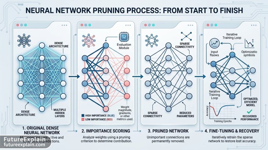
Pruning works in three main steps:
- Train a dense network: First, train a regular neural network to good performance.
- Evaluate importance: Measure how important each parameter (weight) is to the network's output. Common methods include magnitude-based pruning (smaller weights are less important), gradient-based methods, or more sophisticated techniques like Hessian-based pruning.
- Remove and fine-tune: Remove the least important parameters (set them to zero), then fine-tune the remaining network to recover any lost accuracy.
Types of Pruning
Not all pruning is created equal. Different strategies serve different purposes:
- Unstructured Pruning: Removes individual weights anywhere in the network. This creates "sparse" networks with irregular patterns of zeros. While effective at reducing parameter count, it doesn't automatically speed up computation on standard hardware, which is optimized for dense operations.
- Structured Pruning: Removes entire neurons, channels, or layers. This creates smaller but dense networks that run efficiently on standard hardware but may remove more capacity than necessary.
- Global vs. Local Pruning: Global pruning compares all weights in the network and removes the smallest ones overall. Local pruning removes weights within each layer independently, preserving each layer's structure.
Practical Example: Pruning a Image Classifier
Let's consider a practical scenario. You've trained a convolutional neural network to classify 100 different types of animals. The model achieves 94% accuracy but has 50 million parameters and runs slowly on mobile devices. After applying magnitude-based pruning (removing 60% of the smallest weights), the model shrinks to 20 million parameters. Accuracy drops to 91%, but after fine-tuning for a few more epochs, it recovers to 93.5%—nearly matching the original accuracy with less than half the parameters.
The key insight here is that the remaining 40% of weights were doing most of the work anyway. The removed weights were like background noise in a conversation—present but not essential to understanding.
When to Use Pruning
Pruning is particularly effective when:
- Your model is significantly over-parameterized for its task
- Memory footprint is your primary constraint
- You have resources for fine-tuning after pruning
- You're targeting specialized hardware that can exploit sparsity
However, pruning has limitations. Aggressive pruning can damage the network's "learning capacity," making further training difficult. Also, the benefits of unstructured pruning only translate to speed improvements on hardware specifically designed to handle sparse computations efficiently.
Quantization: Doing More with Less Precision
If pruning is about removing unnecessary parts, quantization is about representing necessary parts more efficiently. Imagine you're taking notes in a lecture. You don't need to record every word with perfect precision—you capture the essential ideas in a condensed format. Quantization applies this principle to neural networks by reducing the numerical precision of weights and activations.
The Mathematics of Quantization
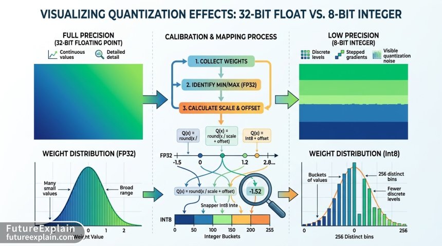
Neural networks traditionally use 32-bit floating-point numbers (float32) to represent weights. Each float32 number requires 32 bits (4 bytes) of memory and can represent values with about 7 decimal digits of precision. Quantization reduces this to lower precision formats:
- 16-bit floating point (float16): 2 bytes per value, ~3-4 decimal digits precision
- 8-bit integer (int8): 1 byte per value, 256 discrete levels
- 4-bit or lower: Even more aggressive compression for extreme constraints
The quantization process involves mapping the continuous range of float32 values to a limited set of discrete integer values. This is done through calibration: analyzing the distribution of values during inference and determining appropriate scaling factors.
Quantization Techniques
Different quantization strategies offer different tradeoffs:
- Post-Training Quantization (PTQ): Quantize a already-trained model without any retraining. Fast but may lose more accuracy.
- Quantization-Aware Training (QAT): Simulate quantization during training so the model learns to compensate. More accurate but requires full training cycle.
- Dynamic Quantization: Quantize weights statically but activations dynamically during inference. Good for models with varying activation ranges.
- Per-Channel vs. Per-Tensor: Per-channel quantization uses different scaling factors for each channel in convolutional layers, preserving more accuracy than per-tensor quantization.
Real-World Impact of Quantization
The benefits of quantization extend beyond just memory savings. Lower precision computations:
- Reduce memory bandwidth: Transferring 8-bit values uses 1/4 the bandwidth of 32-bit values
- Enable hardware acceleration: Many processors have special instructions for 8-bit integer operations that are 2-4x faster than float32
- Lower power consumption: Moving and processing fewer bits uses less energy
A study by Google Research (2021) showed that 8-bit quantization of a BERT language model reduced memory usage by 75% and increased inference speed by 3.5x on mobile CPUs with less than 1% accuracy loss. For edge deployment, these improvements can mean the difference between a feature being feasible or impossible.
When to Use Quantization
Quantization shines when:
- You need inference speed improvements on standard hardware
- Memory bandwidth is your bottleneck
- You're deploying to devices with integer acceleration (like many mobile CPUs)
- You have limited retraining capabilities but need immediate size reductions
The main challenge with quantization is that very low precision (like 4-bit) can cause significant accuracy drops for sensitive tasks. Also, quantization doesn't reduce the number of operations—just their precision—so it doesn't help with compute-bound models as much as pruning does.
Knowledge Distillation: Learning from the Masters
Knowledge distillation takes a completely different approach. Instead of modifying an existing model, it creates a new, smaller model (the "student") that learns to mimic the behavior of a larger, more accurate model (the "teacher"). This is inspired by education: a skilled professor doesn't just give students facts—they convey understanding, intuition, and problem-solving approaches.
The Distillation Process
The key insight of distillation is that a trained model contains more knowledge than just its final predictions. Consider an image classifier that's 95% confident something is a German Shepherd and 5% confident it's a wolf. This "soft probability" distribution contains valuable information: the model sees similarities between these classes. The student model learns from both the hard labels (what the object actually is) and these soft targets from the teacher.
The distillation loss function typically combines:
- Hard loss: Difference between student predictions and true labels
- Soft loss: Difference between student and teacher probability distributions
- Temperature scaling: A parameter that controls how "soft" the teacher's probabilities are
By learning from the teacher's nuanced understanding, the student often achieves better performance than if it had been trained on hard labels alone. This is particularly valuable when the training data is limited or noisy.
Architectural Considerations
Distillation allows for architectural changes beyond just size reduction. The student model can have:
- Fewer layers: Shallower networks with similar width
- Narrower layers: Same depth but fewer neurons per layer
- Different operations: Replacing complex operations (like attention) with simpler alternatives
- Specialized architectures: Designs optimized for specific hardware
A famous example is DistilBERT, which has 40% fewer parameters than BERT but retains 97% of its language understanding capabilities while being 60% faster. The student architecture was carefully designed to preserve the most important aspects of the teacher while removing less critical components.
When Distillation Outperforms Other Methods
Distillation is particularly powerful when:
- The teacher model has learned subtle patterns not captured in the training labels
- You want to change the model architecture significantly (not just shrink it)
- You have unlabeled data available (the teacher can generate pseudo-labels)
- You're targeting very specific hardware constraints
The main drawback of distillation is that it requires training a completely new model from scratch, which can be computationally expensive. Also, if the teacher model has learned biases or errors, the student will inherit them—and sometimes amplify them.
Combined Approaches: When 1+1+1 > 3
The most effective model compression pipelines often combine multiple techniques. A common strategy is:
- Start with a well-trained teacher model
- Distill knowledge to a smaller student architecture
- Apply pruning to remove remaining redundancy in the student
- Quantize the pruned model for efficient deployment
This combined approach can achieve compression ratios of 10x to 50x with minimal accuracy loss. For example, researchers at MIT and NVIDIA demonstrated a computer vision model compressed 48x through combined pruning, quantization, and Huffman coding (an additional compression technique), achieving mobile deployment with only 0.3% accuracy drop.
Case Study: MobileNet Family
The MobileNet architecture family from Google provides an excellent case study in combined compression techniques. MobileNetV3, one of the most efficient architectures for mobile vision tasks, uses:
- Architectural efficiency: Depthwise separable convolutions that reduce computations
- Neural architecture search: Automated discovery of efficient structures
- Hardware-aware design: Optimizations for specific mobile processors
- Quantization: 8-bit integer operations by default
- Pruning: Automated pruning of unimportant channels
The result is a model that runs real-time object detection on smartphones while using minimal battery. This wouldn't be possible with any single compression technique alone.
Practical Implementation Guide
Now that we understand the theory, let's look at practical considerations for implementing these techniques.
Choosing the Right Technique: Decision Framework
Use this decision framework based on your constraints:
| Primary Constraint | Recommended Technique | Expected Improvement | Implementation Difficulty |
|---|---|---|---|
| Memory footprint | Pruning + Quantization | 4-10x smaller | Medium |
| Inference speed | Quantization + Architecture changes | 2-5x faster | Medium-Hard |
| Accuracy preservation | Knowledge distillation | Similar accuracy, smaller size | Hard |
| Deployment flexibility | Post-training quantization | 2-4x smaller, minimal work | Easy |
| Extreme constraints | Combined all three | 10-50x compression | Very Hard |
Implementation Checklist
For each technique, follow this implementation checklist:
Pruning Implementation:
- [ ] Establish baseline model performance
- [ ] Choose pruning criteria (magnitude, gradient, etc.)
- [ ] Decide pruning ratio (start with 20-30%)
- [ ] Implement iterative prune-retrain cycles
- [ ] Validate accuracy after each cycle
- [ ] Consider structured vs. unstructured tradeoffs
Quantization Implementation:
- [ ] Analyze activation ranges with calibration dataset
- [ ] Choose quantization scheme (per-tensor/channel)
- [ ] Implement quantization-aware training if possible
- [ ] Test on target hardware for speed improvements
- [ ] Validate accuracy on edge cases
Distillation Implementation:
- [ ] Select appropriate teacher model
- [ ] Design student architecture based on constraints
- [ ] Choose temperature parameter (start with T=3-5)
- [ ] Balance hard and soft loss weights
- [ ] Use teacher's intermediate representations if available
Common Pitfalls and Solutions
Even with careful implementation, you might encounter these challenges:
- Accuracy collapse after pruning: Solution - Use smaller pruning ratios and more retraining epochs
- Quantization overflow/underflow: Solution - Adjust calibration range or use per-channel quantization
- Student never matches teacher: Solution - Increase model capacity or use more unlabeled data
- Hardware incompatibility: Solution - Test early and often on target hardware
- Training instability: Solution - Use learning rate warmup and careful initialization
Emerging Trends and Future Directions
Model compression is an active research area with exciting developments:
Differentiable Compression
New techniques treat compression as a differentiable optimization problem, allowing end-to-end learning of compressed models. This includes differentiable pruning masks and quantization parameters that can be learned during training rather than determined heuristically.
Automated Compression
Tools like Neural Magic's DeepSparse and Google's Model Optimization Toolkit are making compression more accessible through automation. These tools can automatically apply appropriate compression techniques based on model characteristics and deployment targets.
Hardware-Software Co-design
The most dramatic efficiency gains come from designing models and hardware together. Apple's Neural Engine, Google's TPUs, and NVIDIA's Tensor Cores are examples of hardware designed with compressed models in mind, offering order-of-magnitude improvements over general-purpose hardware.
Extreme Compression for TinyML
For microcontroller-class devices (like Arduino), researchers are pushing compression to its limits with techniques like binary/ternary networks (weights are -1, 0, or 1) and sub-8-bit quantization. The TinyML movement is making AI possible on devices with just kilobytes of memory.
Ethical Considerations and Responsible Compression
As with all AI technologies, model compression comes with responsibilities:
- Bias Amplification: Compression can amplify existing biases in models. Compressed models should be evaluated for fairness across demographic groups.
- Transparency: Heavily compressed models can become "black boxes" even to their creators. Maintain documentation of compression techniques and their effects.
- Environmental Impact: While edge AI reduces cloud energy use, widespread deployment of billions of devices has its own environmental cost. Consider the full lifecycle impact.
- Accessibility: Compression makes AI more accessible by enabling on-device processing, but ensure compressed models remain accurate for all users, including those with disabilities.
Always ask: "Are we compressing responsibly?" not just "Can we compress further?"
Getting Started with Model Compression
Ready to try model compression yourself? Here's a practical starting point:
- Start with a pre-trained model from frameworks like TensorFlow Hub or Hugging Face
- Use established tools like TensorFlow Model Optimization Toolkit or PyTorch's built-in quantization
- Begin with post-training quantization—it's the easiest technique with immediate benefits
- Measure before and after on your target metrics: size, speed, accuracy, power
- Iterate gradually—don't try extreme compression immediately
Remember that model compression is as much art as science. Different models, tasks, and hardware respond differently to compression techniques. The key is systematic experimentation and measurement.
Conclusion
Model compression through pruning, quantization, and distillation is transforming where and how AI can be deployed. These techniques move AI from the cloud to the edge—to your pocket, your home, your car, and countless IoT devices. They make AI faster, more private, more accessible, and more sustainable.
As we've seen, each technique has its strengths: pruning removes redundancy, quantization increases efficiency, and distillation transfers wisdom. Used together, they enable AI models that are orders of magnitude smaller yet nearly as capable as their larger counterparts.
The future of AI isn't just about building bigger models—it's about building smarter, more efficient models that work within the constraints of our world. Whether you're deploying a mobile app, an embedded system, or just curious about how AI fits in tiny devices, understanding these compression techniques is essential for the next generation of AI applications.
Visuals Produced by AI
Further Reading
Share
What's Your Reaction?
 Like
1247
Like
1247
 Dislike
23
Dislike
23
 Love
356
Love
356
 Funny
89
Funny
89
 Angry
12
Angry
12
 Sad
8
Sad
8
 Wow
412
Wow
412


















We're seeing about 2-3x speedup with INT8 quantization on our recommendation models, but the calibration process is tricky with sparse activation patterns. Any tips for models with ReLU6 activations?
Zariyah, for ReLU6 activations, you can use asymmetric quantization with a fixed range of [0, 6] instead of dynamic range estimation. This often gives more stable results. Also consider using percentile-based calibration (e.g., 99.9th percentile) instead of min/max to handle outliers in the activation distribution.
I appreciate the balanced view on tradeoffs. Too many tutorials promise "no accuracy loss" which just isn't realistic for significant compression. Managing expectations is key.
The distillation section could use more examples beyond NLP. In computer vision, we've had success distilling Transformer models to efficient CNNs. The temperature parameter is crucial - too high and you lose detail, too low and it's just copying.
Has anyone compared TensorFlow's quantization tools vs PyTorch's? We're deciding which framework to standardize on for edge deployment.
Hailey, we've used both extensively. TensorFlow Lite has more mature quantization tools with better hardware support (especially for Android). PyTorch Mobile is catching up quickly though, and their quantization-aware training is more flexible. If you're targeting diverse hardware, TF Lite might be safer. For research flexibility, PyTorch.
As a student new to ML, this article connected many dots for me. The decision framework in section 8 is going straight into my notes. Thank you for making this accessible!
The MobileNet case study was eye-opening. We've been using MobileNetV3 in production for six months, and the efficiency gains are real. Battery consumption reduced by 40% compared to our previous custom CNN.